Research shelf / Mathematics / QGO
Written Updated
A QAOA pipeline with no quantum computer and no advantage claim
The usual approach to quantum graph optimisation is to build a QAOA circuit, run it on hardware, and hope the noise does not swamp the signal. This pipeline takes the opposite bet: stay classical, treat noise as a usable signal rather than a nuisance, and make every layer auditable with its own error bookkeeping.
Code exists and runs. Performance not independently checked.
Five auditable layers — spectral compression, Chebyshev encoding, simulated QAOA, noise-weighted ranking, spectral lift-back — each with a named verification function and an explicit error term.
The graph is first compressed spectrally: rank-k truncation of the normalised Laplacian L̃ = I − D−½AD−½, recording relative-Frobenius-tail reconstruction error. A Chebyshev encoder then produces the ansatz with scale 2/λmax and error O(exp(−Jδ/λmax)), so the simulated quantum state starts biased toward the Laplacian’s leading subspace — a graph prior, before any optimisation.
The simulator runs QAOA-style γ-phase and Pauli-X mixing layers on the compressed 2k-dimensional space with depolarising noise, exact below a cap of 18 qubits and mean-field above. The distinctive layer is the noise-aware ranker: shots are down-weighted by w = exp(−λ‖η‖), where η is the bit-marginal deviation between noisy and noiseless Born probabilities. Noise becomes side data instead of error.
Finally spectral lift-back returns to the original graph via z = sign(Uzk), with a verified inequality C(z) ≥ Ck(zk) − εlift|E| bounding what the compression cost. Every layer ships a named verification function — verify_eckart_young, verify_chebyshev_convergence, verify_noise_weighting, verify_liftback_quality, verify_noise_side_data — plus a full-pipeline demo on a Barabási–Albert graph at n = 80.
Every number, and what stands behind it
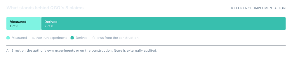
A claim is only worth the evidence attached to it. Each row below carries its basis: measured on the author’s own hardware, derived from the construction, measured on synthetic data, projected from literature, or simply cited.
| Claim | Figure | Basis | Context |
|---|---|---|---|
| Pipeline layers | 5, each independently verified | Derived | Compression, encoding, simulation, ranking, lift-back |
| Compression bound | Eckart–Young optimality | Derived | Verified in code by verify_eckart_young |
| Chebyshev convergence | O(exp(−Jδ/λ_max)) | Derived | With scale 2/λ_max |
| Lift-back guarantee | C(z) ≥ C_k(z_k) − ε_lift|E| | Derived | Verified inequality, not an estimate |
| Exact simulation cap | MAX_EXACT_QUBITS = 18 | Derived | Mean-field approximation above it |
| Noise penalty default | λ = 3.0 | Derived | Weight w = exp(−λ‖η‖) on each shot |
| Parameter grid | 10 × 7 default | Derived | γ-phase and mixing-angle sweep |
| Demo graph | Barabási–Albert, n = 80 | Measured | Cut-fraction and planted-partition comparisons |
Measured — author-run experiment on the stated setup. Synthetic — measured, but on synthetic rather than real data. Derived — follows from the stated construction or proof. Projected — paper-stated projection, not an author-run benchmark. Cited — taken from external literature.
How it works
- Spectral compression. Rank-k truncation of the normalised Laplacian, with reconstruction error recorded rather than assumed small.
- Chebyshev ansatz prior. Amplitude-embedded normalised Chebyshev vector — the graph structure enters before optimisation begins.
- Noise-norm shot weighting. High-‖η‖ shots down-weighted, turning hardware noise into an aggregation signal.
- Verified spectral lift-back. Return to the full graph with an explicit, code-checked bound on what compression cost.
What it does not do
Taken from the folder’s own README. Nothing here has been softened.
- Fully classical. No quantum hardware execution anywhere in the pipeline, and no quantum-advantage claim.
- Compression yields approximate solutions on G_k for G. The lift-back bound quantifies the gap; it does not close it.
- Empirical results are demo-level — one BA(80,4) graph and planted-partition comparisons, not a benchmark suite.
- The "Theorem N" labels are software-documentation conventions backed by in-code tests, not external publications. The README says so.
- Above 18 qubits the simulator is mean-field, so the largest cases are the least exact.
Free under AGPL-3.0+ for almost everyone
Personal use, charities, education and organisations under AUD 50,000 a year pay nothing. A tiered commercial licence covers everyone else.