Research shelf / Software & languages / Statistical Scheduler
Written Updated
A cluster scheduler with three controllers and a regret bound
Most schedulers pick one control philosophy and live with its blind spot. This one runs three: a statistical Completely Fair Scheduler variant for fairness, a Linear Thompson Sampling bandit that learns which node placements actually work out, and a discrete-time PID controller holding load balance. Each carries its own guarantee, and the paper proves them separately before measuring the whole.
Experiments were run and the numbers are reported here.
Fairness from a statistical CFS variant, placement quality from a contextual bandit, load balance from a PID loop — with formal guarantees for each and sub-millisecond measured placement latency.
The scheduler is an asynchronous Python framework for heterogeneous compute clusters. Fairness is handled by a statistical variant of Linux’s CFS; placement quality by Linear Thompson Sampling, a contextual bandit that treats each placement as an arm and learns from realised outcomes; and load balance by a discrete-time PID controller whose stability is argued in the bounded-input-bounded-output sense.
A companion monitoring subsystem watches the cluster with three classical instruments: Holt–Winters triple exponential smoothing for seasonal forecasting, Page–Hinkley CUSUM for change-point detection, and EWMA-based adaptive thresholding. The change detector is characterised the way a control engineer would characterise it — detection latency at a given shift size, against average run length under the null.
The evaluation is 500 scheduling decisions on a 16-node simulated cluster. It reports p50 and p99 placement latency, placement rate, and a Jain fairness index, alongside the theoretical O(d√T · polylog T) regret bound for the bandit. All source is released open.
Every number, and what stands behind it
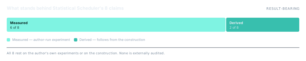
A claim is only worth the evidence attached to it. Each row below carries its basis: measured on the author’s own hardware, derived from the construction, measured on synthetic data, projected from literature, or simply cited.
| Claim | Figure | Basis | Context |
|---|---|---|---|
| Median placement latency | p50 = 0.48 ms | Measured | 500 decisions, 16-node simulated cluster |
| Tail placement latency | p99 = 1.00 ms | Measured | Same run |
| Placement rate | 100% | Measured | Under the representative load tested |
| Jain fairness index | 1.00 | Measured | Perfect on this workload; see limitations |
| LinTS regret bound | O(d√T · polylog T) | Derived | Standard contextual-bandit analysis |
| Change-point detection latency | 3 samples at +3σ | Measured | Page–Hinkley CUSUM, median |
| Average run length under the null | ARL₀ = 3,485 steps | Measured | False-alarm rate of the detector |
| PID stability | BIBO | Derived | Argued, not proved for the closed loop with the bandit |
Measured — author-run experiment on the stated setup. Synthetic — measured, but on synthetic rather than real data. Derived — follows from the stated construction or proof. Projected — paper-stated projection, not an author-run benchmark. Cited — taken from external literature.
How it works
- Statistical CFS. A distributional variant of the Completely Fair Scheduler, supplying the fairness term.
- Linear Thompson Sampling. Contextual bandit over placements, with posterior sampling driving exploration and a standard regret bound.
- Discrete-time PID. Classical proportional-integral-derivative control on the load-imbalance signal.
- Holt–Winters + CUSUM + EWMA. Forecasting, change detection and adaptive thresholding as three separate monitoring instruments.
What it does not do
Taken from the folder’s own README. Nothing here has been softened.
- A Jain index of 1.00 and a 100% placement rate mean the workload was not stressful enough to separate the policies. Both numbers are ceilings, not achievements.
- A 16-node simulated cluster is a simulation. No results on real heterogeneous hardware or on adversarial load.
- The BIBO argument covers the PID loop in isolation. The closed loop formed by PID plus a learning bandit is not analysed for stability.
- The regret bound is the standard LinTS result imported, not re-derived for this setting.
- ARL₀ = 3,485 is one operating point. The full detection-latency/false-alarm trade-off curve is not given.
Free under AGPL-3.0+ for almost everyone
Personal use, charities, education and organisations under AUD 50,000 a year pay nothing. A tiered commercial licence covers everyone else.